

PLEASE READ : THIS PAGE CONSISTS OF HIGHWAY ENGINEERING GATE SYLLABUS (ALMOST ALL THE REQUIRED TOPICS) STUDY MATERIAL COLLECTED FROM DIFFERENT SOURCES (TEXT BOOKS AND MATERIALS OF SEVERAL INDIAN AUTHORS). WE TRIED OUR LEVEL BEST TO BE MAKE THIS MATERIAL CLEAR AND UNDERSTANDABLE TO ANY KIND OF STUDENT. IN CASE YOU FIND ANY MISTAKE IN THIS ONLINE MATERIAL, KINDLY DROP US A NOTE TO OUR EMAIL (civilenggforall@gmail.com) WE WILL BE POSTING THE MATERIALS SIMILARLY TO OTHER SUBJECTS VERY SOON FOR THE BENEFIT OF STUDENTS PREPARING FOR GATE . THIS MATERIAL CONSISTS OF THEORY, SO KINDLY SOLVE THE PROBLEMS AS MANY AS POSSIBLE WITH THE HELP OF THE INFORMATION PROVIDED BELOW.
DOWNLOAD LINK OF THIS MATERIAL (PDF FORMAT) HAS BEEN PROVIDED AT THE END OF THIS POST

HIGHWAY ENGINEERING GATE STUDY MATERIAL CIVIL ENGINEERING FOR ALL EXCLUSIVE
GEOMETRIC DESIGN OF HIGHWAYS
Design Speed: Speed of the vehicle on the road, that should be considered for designing various design features. Design speed can be ruling design speed (usually considered speed) or minimum speed. It usually varies from 20 kmph to 100 kmph.
Highway cross-section elements
(a) Pavement Surface Characteristics
(i) Friction (Skid resistance):
- It is used to calculate design speed, radius of curves, super elevation, sight distances, etc.
- Two phenomena occurring due to friction are skid and slip. Skid occurs when wheel moves without rotating. Slip occurs when wheel rotates more than its corresponding longitudinal distance.
- Frictional resistance along the direction of movement of wheel is called longitudinal frictional resistance and perpendicular to it is known as lateral frictional resistance.
- IRC recommends coefficient of longitudinal friction as 0.35 to 0.40 and coefficient of lateral friction as 0.15.
- Frictional resistance decreases with temperature, wear and tear of tyre, tyre pressure, load, smoothness of pavement and wetness of pavement.
Variation of longitudinal coefficient of friction (f) with speed
| Speed (empty) | f |
| 20 – 30 | 0.4 |
| 40 | 0.38 |
| 50 | 0.37 |
| 60 | 0.36 |
| 80-100 | 0.35 |
(ii) Pavement unevenness:
- It is the cumulative measure of vertical undulation of pavement surface recorded per unit horizontal distance of road.
- It is measured by bump indicator or roughometer and is expressed in terms of unevenness index and unit is usually cm/km.
- Lesser the value, better the pavement.
- For good pavements, it should be 150 cm/km and 250 cm/km is considered satisfactory.
(b) Camber or Cross-slope
It is the slope provided along transverse direction for drainage of rain water from road surface and preventing from seepage to layers below surface and water logging.
- It is expressed as 1 in n or as percentage.
- Depending on shape it can be parabolic, elliptic, straight line or combination of straight line and parabolic.
- Parabolic/elliptical camber
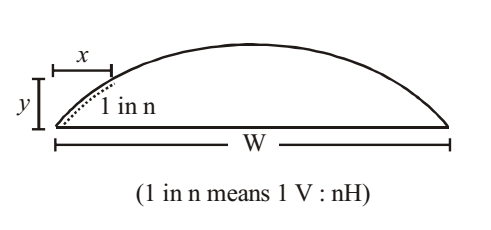
Equation of design : y=2x2/nw
- It is most preferred
- It is good for fast moving traffic
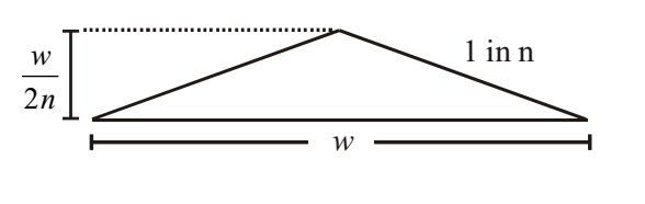
2. Straight line camber:
Height at centre = w/2n
- preferred for cement concrete pavement.
- used when divider is there at the centre of road or on curved road.
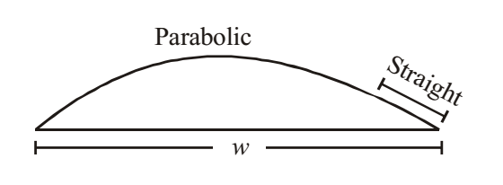
3. Combination of straight and parabolic shape
- has advantages of both parabolic and straight roads
- useful to increase contact area of wheel
- parabolic at centre and straight at both sides.
Recommended values of camber for different roads as per IRC.
| Type of Road | Range of Camber in areas of rainfall range | |
| Heavy | Light | |
| Cement, concrete and high type bituminous surface | 1 in 50 (2%) | 1 in 60 (1.7%) |
| Thin bituminous surface | 1 in 40 (2.5%) | 1 in 50 (2%) |
| Water bond macadam, gravel pavement | 1 in 33 (3%) | 1 in 40 (2.5%) |
| Earth Road | 1 in 25 (4%) | 1 in 33 (3%) |
Tips: Note that camber on light rainfall area of each road is equal to camber in heavy rainfall area just above it.
Points to be noted
- Camber (C) of road is usually given half of longitudinal gradient (G); C=G/2
- Superior the road, flatter will be the camber.
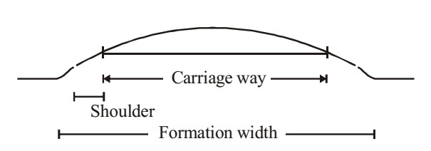
(c) Width of pavement or carriage way
- Width of pavement depends on width of each lane and number of lanes
- Number of lanes depends on predicted traffic volume and capacity of each lane
- Maximum width of vehicles as per IRC is 2.44 m.
Width of carriage way (as per IRC)
| Class of carriage way | Width |
| Single road | 3.75m |
| Multi lane pavements | 3.5m per lane |
| Two lane (without raised kerb) | 7m |
| Two lane (with raised kerb) | 7.5m |
| Intermediate carriage way | 5.5m |
Points to be noted
- Width of single lane roads/village roads is decreased to 3 m and urban roads without kerb to 3.5m
- Minimum width recommended for urban roads with kerb is 5.5 m
(d) Road margins
Various elements of margins are:
- Shoulders: Provided to serve as an emergency lane. Minimum width recommended is 2.5 m.
- Frontage roads
- Drive ways
- Parking lane
- Footpath
- Guard rail etc.
(e) Width of road way or formation
Formation width = carriage way width including separations, if any +shoulder
| Type of Road | Plain and rolling terrain | Mountain or steep terrain |
| NH and SH Single LaneDouble Lane | 12m 12m | 6.25m 8.80m |
| Major District Road (MDR) Single and double lane | 9m | 4.75m |
| Other District Road (ODR) Single laneDouble lane | 7.5m 9m | 4.75m |
| Village Road/Single lane | 7.5m | 4m |
| Single lane bridge | 4.25m | – |
(f) Right of way
Area acquired for road, along its alignment. It depends on the number of lanes, importance of road and future development.
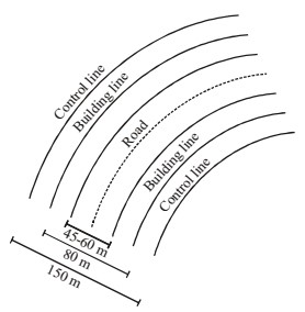
Right of way = Formation width + Road margins.
- NH and SH
Normal width = 45m
Maximum width = 60m
- Distance between
Building line = 80m
Control line = 150m
MADE EASY TRANSPORTATION ENGINEERING GATE NOTES : CLICK HERE
SIGHT DISTANCES
It is the length of road visible ahead to the driver of a moving vehicle at various instances. There are mainly five sight distances considered.
- Stopping Sight Distance (SSD)
- Overtaking Sight Distance (OSD)
- Sight Distance at Intersections
- Intermediate Sight Distance (ISD)
- Head Light Sight Distance
- Stopping Sight Distance (SSD)
It is the minimum sight distance visible to a driver at any instance, that has sufficient length to stop the vehicle travelling at design speed without any chances of collision.
- It depends on feature of road ahead, height of driver’s eye, height of object above road surface, efficiency of brake.
- IRC suggests height of driver’s eye level as 1.5 m and height of obstacle as 0.15 m (15 cm).
- SSD is given by: SSD = Lag distance (L) + Breaking distance (B)
- Lag distance is distance travelled during reaction time. It is based on PIEV theory (Perception, Intersection, Emotion, Volition).
- Usually reaction time is taken as 2.5 seconds.
- Lag distance = reaction time x design speed = t x v
Breaking distance B = v2/2gf
Where v = velocity in m/s
f = longitudinal coefficient of friction
therefore, SSD = Vt + v2/2gf
V is in m/s
SSD = 0.278Vt + v2/2gf
V is in m/s
SSD = 0.278Vt + v2/254f
V is in kmph
SSD at sloping road –
SSD = 0.278Vt + v2/2g(f±0.01n)
or 0.278Vt + v2/254(f±0.01n)
where + is for ascending slope and – is for descending slope
n is the gradient percentage
SSD at level surface with braking efficiency, η
SSD = Vt + V2/2gfη or 0.278Vt + V2/254fη
IRC recommended minimum SSD values
| Design Speed (kmph) | 20 | 30 | 40 | 50 | 60 | 80 | 100 |
| Minimum SSD (m) | 20 | 30 | 45 | 60 | 80 | 120 | 180 |
Points to be noted
- For sloping ground replace ‘f’ by (f±0.01n) and for braking efficiency, η multiply ‘f’ with ‘η’.
- In case of sloping ground and braking efficiencies, denominator becomes 2g(f±0.01n)xη
- SSD for single lane 1-way traffic = minimum SSD (found out by above equation)
- SSD for single lane 2-way traffic = 1/3 x minimum SSD
- SSD for two lane 2-way traffic = minimum SSD
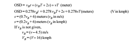
2. Overtaking Sight Distance (OSD)
It is the minimum sight distance visible to a driver intending to overtake a slow moving vehicle with safety against collision with traffic from opposite direction. Or, it can be defined as the distance with his eye level at 1.2m above road surface from where he can see top of an object.
A = Overtaking vehicle
B = Overtaken vehicle
C = Oncoming vehicle
d1 = distance travelled by A during reaction time
d2 = distance travelled by A during overtaking
d3 = distance travelled by C during overtaking
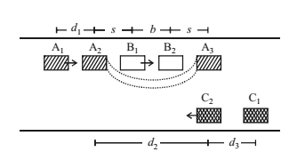
d1 = vBt
t = reaction time (2.5 seconds)
d2 = b + 2s = vBT +2s
T = Time for overtaking
d3 = vT
T = √4s/a sec (a = acceleration in m/s)
OSD = d1 + d2 + d3
Overtaking accelerations as per IRD
| Velocity, V kmph | 25 | 30 | 40 | 50 | 65 | 80 | 100 |
| a m/s2 | 1.41 | 1.3 | 1.24 | 1.11 | 0.92 | 0.72 | 0.53 |
3. Sight Distance at Intersection
At uncontrolled intersections, there should be sufficient visibility at least equal to SSD of the roads.
IRC recommended sight distances at intersections
| Velocity, V kmph | Minor Roads | 60 | 65 | 80 | 100 |
| a m/s2 | 15 | 110 | 145 | 180 | 220 |
4. Intermediate Sight Distance
In cases where OSD cannot be given, ISD is provided to give limited overtaking opportunities to fast-moving vehicles.
5. Head Light Sight Distance
It is the sight distance visible to a driver during night under illumination of front head lamps. This is critical at gradients.
Points to be noted
- For two way traffic, OSD = d1 + d2 + d3
- For one way traffic, OSD = d1 + d2 (as there is no vehicle C)
- Minimum length of overtaking zone = 3 times OSD = 3 × OSD = 3 (d1 + d2 + d3) (2 way) = 3 (d1 + d2) (1 way)
- Usually 5 times OSD is preferred for overtaking zones.
- OSD at grades should be taken more than OSD at level surface.
HIGHWAY ENGINEERING IES MASTER GATE MATERIAL : CLICK HERE
HORIZONTAL CURVES
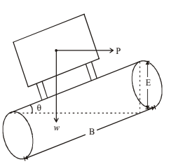
Consider a vehicle moving on a flat road without any super elevation while negotiating a curve.
Centrifugal force acting on the vehicle,
P = mV2/R = wv2/gR
Where m = mass of the vehicle
w = weight of the vehicle
R = radius of the curve (m)
V = velocity of vehicle (m/s)
P/w = V2/gR
Rates P/w is called centrifugal ratio or impact factor
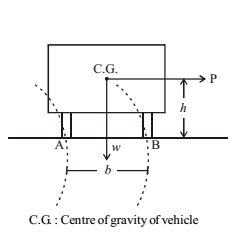
A vehicle negotiating a horizontal curve has two effects based on the centrifugal force. Either the vehicle has the tendency to overturn about the outer wheel (here wheel B) or it has the tendency to skid laterally outwards the road surface (in direction AB)
At equilibrium,
Ph = w.b/2
- P/w = b/2h
(i) Tendency to overturn
At this condition, wheel A just lifts from the surface, i.e., pressure at A = 0
To avoid overturning, centrifugal ratio should be less than b/2h
i.e., P/w or v2/2g < b/2h
Note: To reduce tendency to overturn, while designing a vehicle ‘b’ should be more and ‘h’ should be less, i.e., the vehicle should be broader with lesser height. You might have seen that some of the sports cars are designed so.
(ii) Tendency to lateral skidding
Centrifugal force, P = f × w
where, f = coefficient of lateral friction (≈0.15)
To avoid lateral skid, centrifugal ratio should be less than ‘f’ i.e., P/w or v2/2g < f
Points to be noted
- If f < b/2h, the vehicle skids before it overturns.
- If f > b/2h, the vehicle overturns before it skids.
- To avoid both skidding and overturning, the centrifugal ratio should be less than b/2h and f
SUPER ELEVATION
We have already discussed that in order to avoid of skidding and overturning, p/w should be less than b/2h and f. To reduce the value of centrifugal ratio p/w, we have to reduce the value of centrifugal force, p. This can be done by raising the outer edge of the road with respect to the inner edge. This transverse slope is called super elevation or banking or cant.
Rate of super elevation,
e = tan θ ≈ sin θ = E/B (since θ is small, tan θ ≈ sin θ)
Total height to be elevated, E = e.B
General equation of super elevation is,
e + f = v2/9R (v in m/s and R in m)
= V2/127R (V in kmph and R in m)
At equilibrium super elevation (f=0),
e = v2/9R = V2/127R
Maximum Super Elevation (emax)
- Plain and rolling terrain, snow bound hill terrain : 1 in 15 or 7%
- Hill terrain without snow bond : 1 in 10 or 10%
Design of Super Elevation
(i) For all practical cases, we design for mixed traffic, i.e., e = 0.75v2/9R = V2/225R
(ii) Check the calculated value of e with emax value and the smaller of these two is considered.
(iii) Calculate the value of f with the design speed and maximum super elevation values
f = [V2/127R -emax] = [V2/127R – 0.07] (0.1 for hill terrain)
If the value is less than 0.15 then the value of e is 0
If the value of f is more than 0.15, restrict the speed at the horizontal curve. Restricted design speed is designed as follows.
(iv) emax + f = V2/127R
0.07 + 0.15 = V2/127R (give 0.1 instead of 0.07 for hill terrain)
Thus the allowable speed can be found out.
Points to be noted
- At equilibrium super elevation, pressure on both wheels will be equal. Without super elevation pressure on outer wheel will be more.
- Allowable velocity of vehicle on horizontal curve with super elevation,
V = √(127(e+f)R)
Without super elevation
V = √127fR
- While designing horizontal curves, both minimum super elevation and camber are calculated and the larger of the two is provided.
- For designing super elevation on mixed traffic, only 75% of design speed is taken (i.e., 0.75v instead of V) and lateral friction is neglected. i.e.
e = 0.75v2/9R = 0.75V2/127R = V2/225R
- Ruling minimum design radius and absolute minimum design radius of horizontal curve can be calculated from the equation by substituting values of ruling design speed and minimum design speed, respectively.
e + f = V2/127R
R = V2/127(e+f)
- To attain super elevation, the crown of the camber is eliminated and the edges of pavement are rotated gradually to attain the maximum designed super elevation.
EXTRA WIDENING
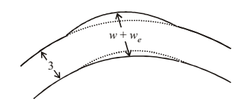
It is the extra width provided at horizontal curves. It is usually provided for curves of radius less than 300m.
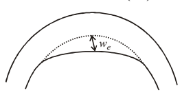
Total widening, We = Wm + Wps
Wm = Mechanical widening
Wps = psychological widening
Wm = nl2/2R
Where l = length of wheel base (≈6m)
n = number of lanes
Wps = V/9.5√R where V is in kmph
We = nl2/2R + V/9.5√R
IRC Recommended values for extra widening
| Radius of curve (m) | upto 20m | 21-40 | 41-60 | 61-100 | 101-300 | >300 |
| Double lane | 1.5 | 1.5 | 1.2 | 0.9 | 0.6 | Nil |
| Single lane | 0.9 | 0.6 | 0.6 | Nil | Nil | Nil |
Points to be noted
- For curves of radius less than 50 m, extra widening is provided only on the inner side of curve.
- For curves of radius more than 50 m, extra widening is provided equally on both sides (We/2)
TRANSITION CURVES
It is provided between straight and circular curves to gradually introduce the curve, super elevation and extra widening.
Types of transition curves
(i) Spiral or clothoid (ideal transition curve)
Length of transition curve α 1/radius
L α 1/R
L.R = consant
(ii) Cubic parabola
(iii) Cubic spiral
(iv) Bernoulli’s Lemniscate
Length of Transition curve (Ls)
It is designed based on three conditions
(i) Rate of change of centrifugal (radial) acceleration (c)
Ls = v3/cR (v in m/s)
c = 80/(75+V) (V in kmph)
0.5 < c < 0.8
(ii) Rate of change of super elevation
Ls = e(ω+ωe)N (pavement rotated about inner edge)
Ls = e(ω+ωe)N/2 (pavement rotated about centre line)
where e = rate in super elevation and N = rate of change of super elevation
(iii) Empirical formulae
Ls = 2.7V2/R for plain and rolling terrain
Ls = V2/R for mountainous and steep terrain
Points to be noted:
- For finding the length of transition curve, the three values are found out and the highest one is taken.
- Shift of transition curve, S = Ls2/24R
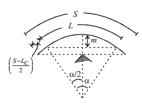
SETBACK DISTANCE
It is the distance between central line of road and an obstruction on the inner side of the curve to provide sufficient sight distance.
(i) It length of curve greater than sight distance (L>S)
Single lane road
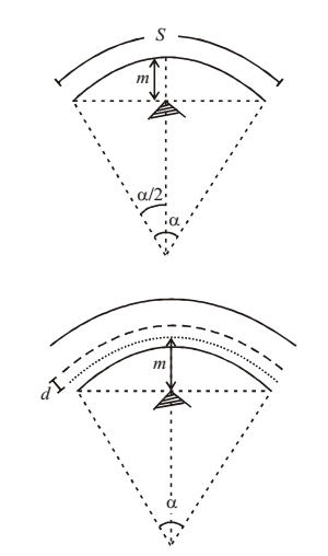
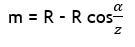
α = S/R (angle = arc/radius)
Note : m ≈ S2/8R’
Multilane road
α = S/(R-d)
where d = distance between central line of road and centre of inner road
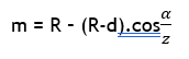
(ii) Length of curve less than sight distance (L<S)
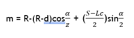
CURVE RESISTANCE
Loss of resistance force due to the turning of vehicle in horizontal curve = (T-Tcosα)
where α is the turning angle and T is actual fracture force
VERTICAL CURVES
GRADIENTS
- Ruling gradient: Maximum gradient used to design a vertical profile of a road.
Rolling terrain – 1 in 30
Mountainous terrain – 1 in 20
Steep terrain – 1 in 16.7
- Limiting gradient: When the gradient is provided steeper than the ruling gradient due to the topography of the area.
- Exceptional gradient: In some exceptional cases, steeper slopes than limiting gradient need to be provided. But exceptional gradient should not be provided for more than 100 m at a stretch. It will be maximum of 1 in 15 for plain terrain.
- Minimum gradient: Gradient to be provided for all roads in drainage point of view. Usually 1 in 500 in considered.
GRADE COMPENSATION
If a steep horizontal curve is to be introduced on a road which already has a gradient of maximum permissible value, then the gradient should be decreased to compensate for the loss of fracture resistance due to the curve. This reduction in gradient is called grade compensation.
% Grade compensation = (30+R)/R
Maximum value of grade compensation = 75/R
where R is radius of curve
Note : Grade compensation need not be considered for gradient flatter than 4%
LENGTH OF VERTICAL CURVES
Usually square parabolic shape is adopted for summit curve and cubic parabola for valley curve.
Length of vertical curve = Total change in gradient/Rate of change of gradient
Equation of curve : y=Nx2/2L
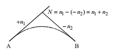
SUMMIT CURVE
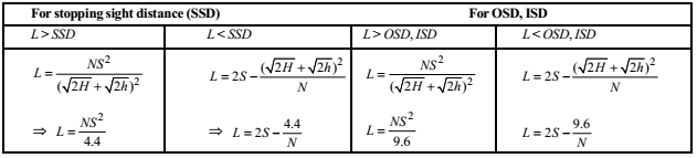
where
L = Length of curve
S = SSD, OSD, ISD
N = Deviation angle
H = Height of eye level of driver above road surface (=1.2m)
h = Height of obstacle above road surface (0.15m)
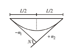
VALLEY CURVE
Valley curve is usually made by two similar transition curves. Valley curve is designed based on two conditions.
a. Comfort condition
b. Head light sight distance
COMFORT CONDITION
Length = 2 x Ls
Where, Ls = Length of one transition curve
Ls = V3/CR
R = Ls/N = L/2N
C = 80/75+V where V is in kmph
0.5 < C < 0.8
Therefore, L = 2Ls = 2[NV3/C]1/2
where N = Deviation angle
C = 0.61 m/s3 (rate of change of centrifugal acceleration)
V is in m/s
L = 0.38[NV3]1/2
Where V is in kmph
Points to be noted
Minimum radius of summit curve, R = L/N
The highest point of summit curve is at distance of Ln1/N from tangent point of n1(A)
HEAD LIGHT SIGHT DISTANCE
1. L > SSD
L = NS2/(2h1 + 2S tanα) = NS2/(1.5 + 0.035S)
where h1 = average height of head light = 0.75m
α = beam angle (≈1o)
2. L < SSD
L = 2S – [(2h1+2S.tanα)/N]
= 2S – [(1.5+0.035S)/N]
Points to be noted
- The longest point of valley curve is at a distance of Ln1/N from the tangent point.
TRANSPORTATION ENGINEERING ACE GATE MATERIAL : CLICK HERE
TESTING AND SPECIFICATIONS OF PAVING MATERIALS
1. Subgrade
The soil fill just below the pavement which receives load from the pavement and gives adequate support.
Important tests
1. Modulus of grade reaction (K) : It is the pressure sustained (P) per unit deformation of subgrade (Δ) at specified pressure or deformation level.
K = P/Δ
Standard plate size = 75cm diameter
Standard settlement = 1.25mm = 0.125cm
K = P/0.125 kg/cm2/cm
2. CBR Test (California Bearing Ratio)
- Used for evaluating stability of soil subgrade and other flexible pavements
- CBR Test apparatus: Cylindrical mould – 150 mm diameter, having base plate and collar Cylindrical plunger – 50 mm diameter Surcharge weight – 147 diameter
- Load values corresponding to 2.5 mm and 5 mm penetration is recorded
- Standard load values: 2.5 mm penetration – 1370 kg (70 kg/cm2) 5 mm penetration – 2055 kg (105 kg/cm2)
- The measured load value is expressed as percentages of standard load values at respective deformation levels to obtain CBR value.
- CBR% = (Load at 2.5mm or 5mm penetration/Standard load at corresponding penetration) x 100
- Normally CBR value at 2.5 mm penetration is higher than that of 5 mm penetration or else the test is repeated.
CBR2.5mm > CNR5mm
2. Stone Aggregates
Characteristics of stone aggregates and various tests to measure these properties are discussed below
(i) Strength: Ability of an aggregate to withstand stresses or crushing load under gradually applied compressive load.
Test: Aggregate crushing test
Dry aggregates of sizes between 10 mm and 12.5 mm are taken and filled in the mould in 3 layers and tamped. 40 tonnes of load is applied at a rate of 4 tonnes/minute.
Aggregate crushing value = (Weight of crushed aggregate passing through 2.36 mm sieve × Total weight of aggregate) x 100
= (w2/w1)x 100
IRC Recommendation : Aggregate crushing value
For base course should not be greater than 45%
For surface course should not be greater than 30%
(ii) Toughness: It is the resistance of a material against impact or sudden load.
Test: Aggregate Impact test
Aggregate is taken in the mould in the similar way as in crushing test.
Hammer of 13.5 to 14 kg is allowed to free fall at a height of 38 cm and 15 such blows are given.
Aggregate impact value = (Weight of crushed aggregate retained on 2.36mm sieve/Total weight of aggregate) x 100
= w2/w1 x 100
IRC Recommendations
For wearing course, aggregate impact value should be lesser than 30%
For base course (bituminous macadam), aggregate impact value should be lesser than 35%
For base course (wbm), aggregate impact value should be lesser than 40%
(iii) Hardcore: It is the resistance to abrasion. Different tests are carried out to test abrasion.
(a) Los Angeles Abrasion test:
5-10 kg specimen is taken, and cast iron abrasive charges of 4.8 cm diameter and 390-445 gram weight is used for the test. It is rotated at 30-33 rpm, with a total of 500-1000 revolutions.
Abrasive value = (Weight of aggregate passing through 1.7 mm sieve/Total weight of aggregate) x 100
IRC recommendation:
For cement concrete construction, abrasive value should be less than 16%
For wearing course, abrasive value should be less than 30%
For base course, abrasive value should be less than 50%
(b) Deval abrasion test: Same type of test as above but concluded on a different type of testing machine.
(c) Dorry abrasion test: Similar to that of devel test but abrasive charges are not used. This test is obsolete.
(iv) Weathering action:
Test: Soundness test
Dry aggregate is weighed and is immersed in saturated solution of sodium sulphate (Na2SO4) or magnesium sulphate solution (MgSO4). Average loss of weight of aggregate is measured.
IRC recommendation:
12% when tested with Na2SO4
18%: tested with MgSO4
(v) Shape of aggregate:
Test: Shape test
(a) Flakiness index: Percentage by weight of aggregate whose least dimension is less than 0.6 times mean demension. Test is applicable for aggregate size more than 6.33 mm.
(b) Elongation index: Percentage by weight of aggregate whose greater dimension is greater than 1.8 times mean dimension.
IRC recommendation: Flakiness index < 15%, Elongation index <10-15%
(vi) Specific gravity and water absorption
IRC recommendation:
Specific gravity: 2.6 to 2.9
Water absorption < 0.66%
Angularity number: It is the measure of voids in excess of rounded gravel, for which void ratio is 33%.
Angularity number = 67 – %solid volume = 67 – (100w/C.G)
Where, w = mean weight of aggregate in cylinder, C = weight of water required to fill the cylinder, G = specific gravity of aggregate.
Note: Higher the angularity number, more angular the aggregate. Angularity number is always expressed as nearest whole number. Angularity number is used for construction: 0 to 11.
(vii) Adhesion to bitumen:
Tests used
- Static immersion test (commonly used)
- Dynamic immersion test
- Chemical immersion test
- Immersion mechanical test
- Coating test
IRC recommendation: Stripping value of aggregate
< 5%
BITUMINOUS MATERIALS
- Bitumen is a hydrocarbon obtained by fractional distillation of petroleum.
- If the bitumen contains some inert material, it is called asphalt.
- Jar is obtained by destructive distillation of natural organic materials like wood.
- If the viscosity of bitumen is reduced by any volatile diluent, it is called cut back bitumen.
- If the bitumen is suspended in a finely divided condition in an aqueous medium and stabilized with an emulsifier, it is called an emulsion.
TYPES OF BITUMEN
A type: Eg.: A30, A90
S type: Eg.: S30, S90
Tests on Bitumen:
1. Penetration Test: It is used to determine hardness or consistency of bituminous materials. The distance traversed by standard needle in the bituminous materials is measured in 1/10th of a millimeter. Grading of bitumen is done by this value, e.g. 80/100 means penetration value of bitumen is between 80 and 100. At hot climate 30/40 is preferred.
2. Ductility Test: It is expressed as distance in ‘cm’ to which a standard briquette of bitumen can be stretched before it breaks.
Rate of pull: 50 mm/min or 5 cm/min.
This test measures elasticity and adhesiveness of bitumen. The ductility value usually varies from 5 cm to 100 cm. Desirable value: 50 cm.
3. Viscosity Test: It is used to specify the consistency of bitumen. Viscosity is the resistance of flow of the fluid. It is measured by orifice type viscometer. It is determined by measuring number of seconds required for 50 ml of material to flow through standard orifice.
4. Float Test: It is also used to measure consistency. Float test value is determined by measuring time taken in seconds by water to force its way into the float through the bitumen plug. Higher the value, stiffer the material.
5. Softening Point Test: It is the temperature at which a substance attains a particular degree of softening under standard test conditions. It is usually measured by Ring and Ball test. For high grade bitumen, softening point will be higher and penetration value will be lesser. Bitumen of higher softening point is preferred in warm climate areas.
6. Specific Gravity Test: Specific gravity is determined by a pycnometer. Pure bitumen has specific gravity values ranging from 0.97 to 1.02. Cutback bitumen usually has lower specific gravity. Jar has specific value ranging from 1.10 to 1.25.
7. Flash and Fire Point Test: It is measured by Pensky–Martens apparatus. Flash point is the lowest temperature at which vapour of a substance momentarily catches fire in form of flash. The minimum specified flash point value of bitumen is 175°C. Fire point is the lowest temperature at which the application of test flame causes the material to ignite and burn at least for 5 seconds under specified conditions.
8. Spot Test: It is used to determine overheated or cracked bitumen. Naptha solution is used for this test.
9. Loss on Heating Test: Bitumen is heated to 163°C for 5 hours. The specified value for bitumen used for pavement mixes is that it should not be more than 1%.
10. Solubility Test: Pure bitumen is completely soluble in carbon disulphide (CS2) and carbon tetrachloride (CCl4). Solubility is measured as percentage of original sample that dissolves in these solvents. In test with CCl4, bitumen is considered to be cracked if blank residue is more than 0.5%. In test with CS2, minimum proportion of bitumen soluble should be 99%.
11. Water Content Test: Minimum water content in bitumen should be less than 0.2% by weight.
CUTBACK BITUMEN
It is the bitumen whose viscosity has been reduced by a volatile dilutent. It is used for surface dressing and soil bitumen stabilization particularly at low temperature.
Types of Cutbacks:
1. Rapid Curing (RC): Diluent will rapidly evaporate when used for construction. For RC, petroleum diluent like naptha or gasoline is fluxed to bitumen.
2. Medium Curing (MC): For MC, bitumen is fluxed with intermediate boiling point solvents like kerosene or light diesel oil so that it won’t evaporate faster.
3. Slow Curing (SC): For SC, bitumen is fluxed with high boiling point gas oil.
BITUMINOUS EMULSION
It is prepared by suspending finely divided bitumen in an aqueous medium and adding stabilizers to it. It is used mainly in maintenance repair works and for soil stabilisation. It can be used in wet weather. On application on roads, it break down and binder starts binding the aggregate.
Tar: It is obtained by destructive distillation of wood or charcoal. Tars are of five grades in increasing order of viscosity:
RT-1, RT-2, RT-3, RT-4, RT-5
RT-1 is of the lowest viscosity and is used for surface pointing whereas RT-5 of the highest viscosity is used for grating purposes.
Points to be noted
Suffix numbers 0 to 5 are used to designate definite viscosity of the cutback bitumen with increasing thickness.
Example: SC-3 means slow curing cutback bitumen of grade 3.
Marshall Stability Test:
- Test is applicable to hot mix-paving mixture design using penetration grade bitumen and containing aggregate with maximum size of 2.5 cm.
- It is a type of unconfined compression strength test, in which a cylinder specimen of 10 cm diameter and 6.3 cm height is compressed radially at a constant rate of strain of 5 cm/min.
- Corresponding load carried by specimen at standard temperature (60°C) is called Marshall Stability value and the deformation at failure in units of 0.25 mm is recorded as Marshall flow value.
- The optimum binder content for aggregate mixture and anticipated traffic conditions is a compromise value which meets specified requirements for stability slow value and void content.
Design Specification: Marshall stability = min. 340 kg Flow value (0.25 mm units) = 8-17 Percentage air voids in mix. = 3-5% Voids filled with bitumen = 75-85
DESIGN OF PAVEMENTS
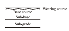
Pavements are classified flexible and rigid pavement based on its structural behaviour. Flexible pavement consists of series of layers with the highest quality material at the top layer to sustain the compressive stresses and wear and tear. Rigid pavement consists of one course of concrete slab which takes up the loads.
Components of pavements:
Wearing course: Gives smooth surface, watertight layer. Base and sub-base: Improves load carrying capacity, transfers load to bottom.
Sub-grade: Natural soil prepared 50 cm thickness recommended.
Tests conducted to test strength: CBR test, California resistance value test, Triaxial test, Plate bearing test.
DESIGN FACTORS
1. Design Life: It depends on type and importance of road. Varies from 15 to 30 years.
2. Design Traffic: It is based on 7 days 2 hours traffic count as per IRC–9. Anticipated traffic,
A = P[1 + r]n
P = last counted no. of vehicles/class
r = rate of growth of traffic (usually 7.5% is taken)
n = number of years
A = P(1.075)n
3. Maximum Wheel Load
- It influences the quality of road surface.
- Pavement design is based on 98th percentile axle load.
- Maximum legal axle load = 8,200 kg (flexible pavement) = 10.2t (rigid pavement)
- Maximum equivalent single wheel load is half of maximum legal axle load.
4. Contact Pressure
- Contact pressure = Load on wheel/Contact area
- Contact area is taken circular in shape.
- Influences quality of surface layer.
- Contact pressure for road vehicles = 5-7 kg/cm2
- Rigidity factor = Contact pressure Tyre pressure
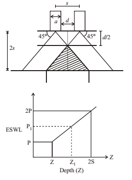
5. Equivalent Single Wheel Load (ESWL): To carry large roads, vehicles are provided with dual wheels. The total load will be less than 2 times load on each wheel. ESWL is calculated by equivalent deflection criterion (more reliable) or equivalent stress criterion.
Equivalent stress criterion is used by the graph of ESWL with depth (Z)
s = d + 2a
a = radius of circular contact area
Repetition of loads: If N1 and N2 are no. of repetition and P1 and P2 are corresponding loads; P1N1 = P2N2 i.e. P α 1/N
Points to be noted
- Rigidity factor = 1 for tyre pressure ≈ 7 kg/cm2
- As tyre pressure increases than 7 kg/cm2 rigidity factor decreases than 1 and vice-versa.
TRANSPORTATION ENGINEERING ACE GATE NOTES : CLICK HERE
DESIGN OF FLEXIBLE PAVEMENTS
1. CBR METHOD (CALIFORNIA BEARING RATIO)
Used to determine the thickness of pavement above the sub-grade irrespective of the material used.
Thickness of pavement (t) (if CBR < 12%)
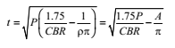
where
P = wheel load (kg)
CBR = CBR%
U = tyre pressure
A = area of contact
2. TRIAXIAL TEST METHOD
Thickness of pavement (t)
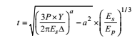
where,
P = wheel load
X = traffic coefficient
Y = saturation coefficient
Es and EP = modulus of elasticity of sub-grade and pavement (t α (1/E)1/3)
Δ = design deflection
a = area of contact
Stiffness factor = (ES/EP)1/3
DESIGN OF RIGID PAVEMENT
Load in a rigid pavement is taken by the slab. The load carrying capacity of slab is due to its rigidity and high modulus of elasticity. This is called slab action.
Radius of Relative Stiffness: The sub-grade below the slab offers some degree of resistance to slab deflection. The slab deflection is measurement of magnitude of sub-grade pressure.
Radius of gyration,
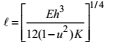
where,
E = modulus of elasticity of concrete
K = modulus of sub-grade reaction
h = slab thickness
u = Poisson’s ratio of concrete (0.15)
Equivalent radius of resisting section (b): It gives the radius of area resisting bending moment of the plate.
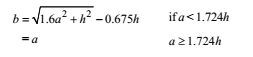
Where a = area of wheel load distribution = √(P/qπ)
Point to be noted: For interior and edge loading, tensile stress is at the bottom of slab, and for corner loading tensile stress is at the top.
1. Wheel Load Stress
It acts not around the load but at a distance ‘x’ from corner bisector
Where x = 2.58√al
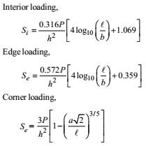
2. Westergaard’s Equation for Wheel Loads
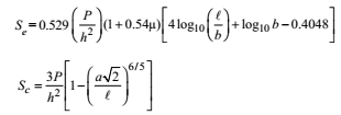
Modified Westergaard’s Equation
3. Temperature Stresses :
Temperature stresses can be due to variation in temperature due to daily variation and seasonal variation
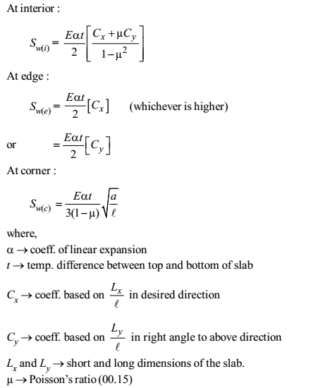
a. Warping Stress: This is due to daily variation of temperature
b. Frictional Stress: It is induced at the bottom of slab due to uniform temperature variation
Force in slab due to movement = Frictional resistance due to sub-grade
- Sf x h x B = [B x L/2 x h].rc.f
Therefore, Sf = rc.f.L/2
where Sf = unit stress developed in slab
L,B = Length and breadth of slab
rc = unit weight of concrete (2400 kg/m3)
f = coefficient of friction ≈ 1.5
CRITICAL STRESS COMBINATIONS
MID DAY
- During Summer : At edge, Scritical = Se + Sw(e) – Sf
- During Winter : At edge, Scritical = Se + Sw(e) + Sf
- Mid-night : At corner, Scritical = SC + Sw(C)
HIGHWAY ENGINEERING CIVILENGGFORALL EXCLUSIVE GATE PSU ESE MATERIAL IN PDF FORMAT : CLICK HERE
PASSWORD : CivilEnggForAll
OTHER USEFUL POSTS
- RAJASTHAN STAFF SELECTION BOARD (RSSB) JUNIOR ENGINEER DIPLOMA CIVIL ENGINEERING EXAM 2022 – HINDI & ENGLISH MEDIUM SOLVED PAPER – FREE DOWNLOAD PDF (CivilEnggForAll.com)
- ISRO TECHNICAL ASSISTANT EXAM 2022 – CIVIL ENGINEERING – HINDI & ENGLISH MEDIUM – SOLVED PAPER – FREE DOWNLOAD PDF (CivilEnggForAll.com)
- MADHYA PRADESH PUBLIC SERVICE (MPPSC) COMMISSION – ASSISTANT ENGINEER EXAM – MPPSC AE 2021 CIVIL ENGINEERING – SOLVED PAPER WITH EXPLANATIONS – PDF FREE DOWNLOAD
- BIHAR PUBLIC SERVICE COMMISSION (BPSC) ASSISTANT ENGINEER EXAM – 2022 – CIVIL ENGINEERING – SOLVED PAPER – FREE DOWNLOAD PDF (CivilEnggForAll.com)
- ODISHA PUBLIC SERVICE COMMISSION – OPSC AEE PANCHAYATI RAJ EXAM 2021 – SOLVED PAPER WITH EXPLANATION – FREE DOWNLOAD PDF