SOIL MECHANICS – ONLINE GATE STUDY MATERIAL

VALUE IN GATE – 15 MARKS

PLEASE READ : THIS PAGE CONSISTS OF SOIL MECHANICS GATE SYLLABUS (ALMOST ALL THE REQUIRED TOPICS) STUDY MATERIAL COLLECTED FROM DIFFERENT SOURCES (TEXT BOOKS AND MATERIALS OF SEVERAL INDIAN AUTHORS). WE TRIED OUR LEVEL BEST TO BE MAKE THIS MATERIAL CLEAR AND UNDERSTANDABLE TO ANY KIND OF STUDENT. IN CASE YOU FIND ANY MISTAKE IN THIS ONLINE MATERIAL, KINDLY DROP US A NOTE TO OUR EMAIL (civilenggforall@gmail.com) WE WILL BE POSTING THE MATERIALS SIMILARLY TO OTHER SUBJECTS VERY SOON FOR THE BENEFIT OF STUDENTS PREPARING FOR GATE. THIS MATERIAL CONSISTS OF THEORY, SO KINDLY SOLVE THE PROBLEMS AS MANY AS POSSIBLE WITH THE HELP OF THE INFORMATION PROVIDED BELOW.

DOWNLOAD LINK OF THIS MATERIAL (PDF FORMAT) HAS BEEN PROVIDED AT THE END OF THIS POST

Soil Mechanics Free Online CivilEnggForAll GATE Study Material

CONTENTS

Origin Of Soils

Soil Classification

Three Phase Diagram

Index Properties Of Soil

Relative Density
Particle Size Distribution
Consistency
Atterberg’s Limits

Engineering Properties Of Soil

Permeability
Seepage
Quick Sand And Piping
Effective Stress
Stress Distribution
Consolidation
Compaction
Shear Strength

ORIGIN OF SOILS (0 Questions asked from last 6 years of GATE)

Soils are formed from weathering of rocks and decomposition of organic matter.
Types of weathering – Physical weathering: by temperature, frost action, abrasion etc. – Chemical weathering: oxidation, carbonation, hydrolysis etc.
Different types of soils – Alluvial soil, Black soil (Cotton soil), Laterite soil, Sandy Soil etc.
Alluvial soil is formed by river transportation, Black soil by chemical weathering and laterite soil by leaching.

SOIL CLASSIFICATION (0 Questions asked from last 6 years of GATE)

How can be soil classified?

Classification based on origin and type of soil
Residual soil: Soil formed by weathering and is deposited there itself.
Transported soil: Soil transported by agents like water, wind, ice, glaciers etc.

Have a look at below types of transported soil and their respective agents.

Types of Soil	Agents of Transportation
Alluvial	Rivers
Lacustrine	Lake
Marine	Ocean
Aeolian (Sane dunes, Loess)	Wind
Drift	Glacier
Till	Melting of glacier
Colluvial (Talus)	Gravitation

THREE PHASE DIAGRAM (BLOCK DIAGRAM) (Minimum 1 Question from this topic in every year GATE Exam)

What are the contents of three phase diagram of soil?

Unsaturated soil consists of solids, water and air which forms the three phase diagram
Basic abbreviations used: Vs, Vw, Va represents volume of solids, water and air respectively V represents total volume.

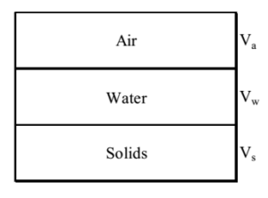
V_{s ,} V_{w ,} V_a represents volume of solids, water and air respectively V represents total volume.

V_v = V_a + V_w

V=V_a + V_w + V_s = V_v + V_s

PROPERTIES

What are the volume relations of soil?

1. Void ratio e = V_v/V_s

Remember volume = weight/density (It can be used to solve some problems)

Value of ‘e’ always greater than zero.
e _{coarse grained} < e _{fine grained}

2. Porosity (η) or percentage voids

η = V_v/V

0 < η < 100%

Relationship between Void Ratio and Porosity

e = η/(1- η)

η = e/(1+e)

3. Degree of Saturation (S_r)

S_r = V_w x 100 / V_v

0 ≤ S_r ≤ 100%

S_r = 0 for dry soil and S_r = 1 for fully saturated soil.

4. Air content (a_c)

a_c = V_a/V_v

a_c = 0 for fully saturated soil and a_c = 1 for dry soil.

Relationship between a_c and S_r is

a_c = 1-S_r or a_c+S_r = 1

5. Percentage air voids (η_a)

η_a = V_a x 100/V

0 ≤ η_a ≤ η

η_a for fully saturated soil and η_a= η for dry soil.

For dry soil, V_w=0 , therefore V_v = V_a

Relationship between η_a, η and a_c is η_a = η x a_c

DENSITY OF SOLID MASS

1. Bulk Density

γ_b= W/V = (W_W+W_S)/V

2. Dry Density

γ_d = W_S/V

3. Density of Solids

γ_S = W_S/V_S

(Unit wt. of solids) γ_s is constant for given soil, but γ_d is not.

4. Saturated density

γ_sat = W_sat/V

5. Submerged density (γ_sub or γ’) = W_sub/V

W_sub is Submerged Weight of Soil

Relationship between γ_sub and γ_sat is γ_sub = γ_sat – γ_wwhere γ_w is density of water

Water Content or Moisture Content W_C = W_W x 100/W_S

W_C > 0

W_W, W_S, W represents weight of water, solids and total weight

SPECIFIC GRAVITY OF SOLIDS

Specific Gravity (G) = γ_S/γ_w

G is measured at 27⁰C

G is usually taken as 2.65

γ_Sis density of soil solids

γ_w is density of water

Apparent/Bulk/Mass Specific Gravity (G_m) = γ_b/γ_w

γ_bis bulk unit weight

G_m < G

For a given soil, G is constant but G_m is not.

Relationship between volume of soil, void ratio and dry density.

V₁/V₂ = (1+e₁)/(1+e₂) = γd₂/γd₁

SHORT-CUT TO STUDY THE PROPERTIES

This is a shortcut method to remember the properties of soil discussed above. Instead of studying the five properties we can just study the diagram given below. The arrow mark means ‘divided by’

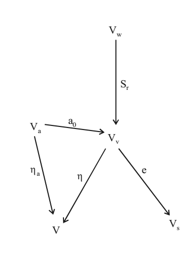
Shortcut to Study the Properties

Example, V_w → V_v means V_w/V_v

The properties are shown nearby the arrows.

Example, S_r = V_w/V_v

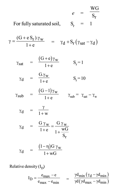
FEW MORE FUNCTIONAL RELATIONSHIPS

Questions are frequently asked in GATE exam from this part. It is better to know all these equations. Also, workout some problems using these equations.

INDEX PROPERTIES OF SOIL

Main index properties of different types of soil are

Coarse grained soil – Relative density, particle size distribution

Fine grained soil – Atter berg’s limits, consistency of soil.

Relative density (I_D) = x 100

e_max is void ratio in its loosest state. (In loosest state, the volume of voids is maximum for unit volume of solids, so void ratio is maximum)

e_min is void ratio in its densest state.

e is void ratio in natural state.

I_D is expressed in percentage. So its value varies from zero to 100.

If I_D is less than 35%, soil is said to be in loose dense state and if I_D is above 85% soil is said to be very dense state.

Another equation of I_D is I_D = γ_dmax(γ_d – γ_dmin)/ γ_d(γ_dmax– γ_dmin)

PARTICLE SIZE DISTRIBUTION

Based on the soil particle/grain size soil can be classified as

GRAIN SIZE (mm)	TYPE
Less than 0.002 mm	CLAY
0.002 – 0.075 mm	SILT
0.075 – 4.75 mm	SAND
4.75 – 80 mm	GRAVEL

POINTS TO REMEMBER

Usually, clay and silt (size < 0.75 mm) is referred as fine grained soil and sand gravel (size > 0.75 mm) is referred as coarse grained soil.
1 mm = 1000 microns (1000 P) Example 0.075 mm = 75 P
For particle size distribution, we use sieve analysis for coarse grained soil (< 75 P) and sedimentation analysis/ wet analysis for fine grained soil (< 75 P).
Sedimentation analysis is based on Stoke’s Law in which the terminal velocity of the particle is found out.

Terminal Velocity, V = d²(γ_s-γ_w)/18µ= 9(S-1)d²/18ν ≈ 902 d²

µ and ν – dynamic and kinematic viscosity of water respectively.

Where, d – diameter of particle and γ_s – unit wt. of particle

Sedimentation analysis can be done either by pipette method or hydrometer method.
In these method, dispersion solution is prepared by adding 33 grams of sodium hexametaphosphate and 7g of sodium carbonate in distilled water.

PARTICLE SIZE DISTRIBUTION CURVE

It is a curve plotted on a semi-log graph which shows the gradation and type of soil. The log of diameter of particle is in the x-axis and the percentage finer is in the y-axis.

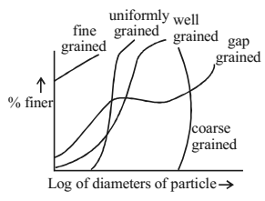
PARTICLE SIZE DISTRIBUTION CURVE

Fine grained – most of the particles are of smaller size
Coarse grained – most of the particles are of gravel size
Uniformly grained – most of the particles are of same size
Well grained – particles of all sizes are present in similar ratio
Gap grained – particles of some sizes are found in even.

IMPORTANT TERMS IN PARTICLE SIZE DISTRIBUTION

Effective size (D₁₀): The size of particle such that only 10% of the particle are less than this size. It is also called effective diameter and is usually represented in mm.

Uniformity coefficient (C_u)

C_u = D₆₀/D₁₀

where D₆₀ means 60% of particles are finer than this size

Coefficient of curvature Cc = D₃₀²/(D₆₀ x D₁₀)

D₃₀ means 30% of particles are less than this size.

Points to be noted

C_u will be always greater than or equal to 1
Uniformly graded soils will have C_u & C_c approximately equal to 1.
Well graded soils will have C_c between 1 and 3
Well graded gravel will have C_u≥ 4 and well graded sand will have C_u≥ 6
Angularity of a particle = (Average radius of corners and edges)/(Radius of maximum inscribed circle)
Based on angularity, particles can be classified as angular, sub angular, sub rounded, rounded, well rounded.

CONSISTENCY

Consistency of a cohesive soil is the physical state in which it exist.
It is mostly used for fine grained soil and denotes the degree of firmness or stiffness of the soil.
The water content at which soil changes from one state to another are known as consistency limits/ Atterberg limits.

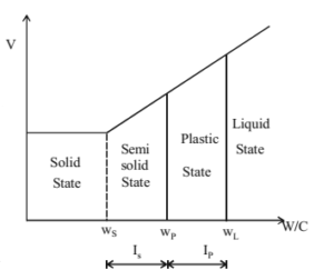
CONSISTENCY LIMIT/ ATTERBERG’S LIMIT

There are four states of consistency depending on the water content – Liquid state, plastic state, semi-solid state, solid state.
There are three limits of water content in which the state of soil changes from one state to another.

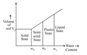
Atterberg’s Limits

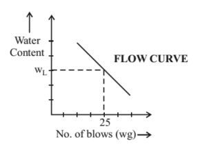
Flow Curve

LIQUID LIMIT (W_L)

It is the minimum water content in which soil is in the liquid state. x Liquid limit is found out using Casagrande’s apparatus.
Using this apparatus we find out the minimum water content at which soil man cut by a grooving tool (as confirm to IS 9259 – 1987) of standard dimension will flow together for a distance of 0.5 inches (12 mm) under impact of 25 blows.
Using Casagrandes’ apparatus, with different water content and finding out no of blows, we get the flow curve.

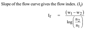
n₁ & n₂ are number of blows corresponding to water contents w₁& w₂.

Shear strength of soil at liquid limit is about 2.7 kN/m2.

PLASTIC LIMIT (W_P)

Minimum water content in which soil turns from plastic state to semisolid state.
It is found out by Thread test.
Water content at which soil when rolled into a thread of 3.18 mm (1/8 of an inch), begins to crumble is called plastic limit.

SHRINKAGE LIMIT (W_S)

Maximum water content at which further decrease in water content cause any reduction in volume of solid mass is called shrinkage limit.
At this limit the soil stops shrinking and volume remains constant. This volume is the day volume of soil (V_d).

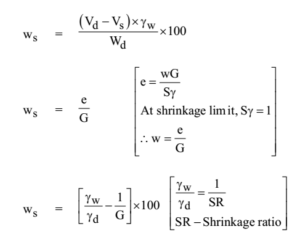
Shrinkage Limit

Shrinkage ratio (SR) – It is defined as the ratio of given volume change, expressed as a percentage of dry volume, to the corresponding change in water content.

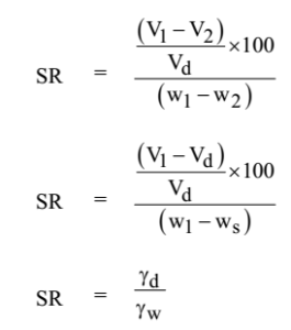
Shrinkage Ratio

SR = G_m (mass specific gravity of soil in dry state)

V₁ – Volume of soil mass at water content w₁

V₂ – Volume of soil mass at water content w₂

V_d – Volume of dry soil mass.

w_s – Shrinkage limit

Volumetric Shrinkage (VS) – It is the change in volume expressed as a percentage of dry volume when water content is reduced from given value to shrinkage limit.

VS = 100(V₁-V_d)/V_d

SR = VS/(w₁-w₂)

Linear Shrinkage (LS) – It is the percentage change in length to actual length when water content is reduced to Shrinkage Limit.

LS = 100(Initial Length – Final Length)/Initial Length

Indices in Atterberg limits

1. Plasticity Index. (I_P)

It is the numerical difference between liquid limit and plastic limit.

It denotes the width of plastic state in water content – volume graph. I_P = w_L – w_P

When I_P = 0, there is no plastic state and soil is said to be non-plastic.

When I_P > 17, soil is said to be highly plastic. Eg: Clayey soil.

2. Shrinkage Index (I_S)

It is the numerical difference between plastic limit and shrinkage limit. I_S = w_P – w_S

It denotes the width of semi solid state in water content-volume graph.

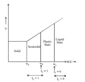
3. Consistency Index/ Relative consistency (I_C)

I_C = (w_L – w)/(w_L – w_P) where w = weigh content of soil

= w_L – w / I_P

Different Cases

When IC = 1, (w_L – w)/(w_L – w_P) = 1 → w_L – w = w_L – w_P → w = w_Pe., soil is in plastic state.
When IC = 0, (w_L – w)/(w_L – w_P) = 0 → w_L – w > 0 → w = w_Le., soil is in liquid state.
When IC > 1, (w_L – w)/(w_L – w_P) > 1 → w_L – w > wL – w_P → w < w_Pe., soil is in semisolid state.
When IC < 0, (wL – w)/(w_L – w_P) < 0 → w_L – w < 0 → w > w_Le., soil is in liquid state (I_C is negative)

Points to be noted

When consistency is less than 50 soil is soft.
When consistency index is greater than 100 soil is very stiff.

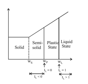
4. Liquidity Index/ Water plasticity ratio (I_L)

I_L = (w – w_P)/(w_L– w_P) = (w – w_P)/I_P

Similar to above, substituting various values for IL.

When I_L= 0, w = w_P i.e., soil is in plastic limit

When I_L = 1, w = w_L i.e., soil is in liquid limit

When I_L > 1, w > w_L i.e., soil is in liquid state

When I_L < 0, w < w_P i.e., soil is in semisolid state I_C + I_L = 1 or 100%

5. Toughness Index (I_T) – Toughness Index is the ratio of plasticity index to flow index

I_T = I_P/I_F

Points to be noted

When particle size decreases, w_L, w_P and I_P is increases
When silt is added to clay, w_L, w_P and I_Pdecreases
As I_T increases, strength of soil in plastic state increases.

Important Terms Related to Consistency

Activity (A) It is the ratio of plasticity index to percentage of clay fraction

A = I_P/ % clay

It is the measure of water holding capacity of clayey soil

If A < 0.75, soil is inactive.

If A is between 0.75 to 1.25, soil has normal activity

If A > 1.25, soil is active

Soil having clay mineral ‘montmorillonite has activity greater than 4

Thixotropy –

What is Thixotropy?

Gaining of strength of soil with passage of time after it has been remoulded is called thixotropy. It is due to gradual reorientation of molecules of water in the absorbed water layer and due to re-establishment of chemical equilibrium.

Sensitivity (S) It is the ratio between unconfined compressive strength of undistributed clay to union final compressive strength of remoulded clay/ soil.

S = UCS of undisturbed soil UCS of disturbed soil

When the soil structure is disturbed the engineering properties of soil changes considerably.

Sensitivity is the ratio of undisturbed strength to remoulded strength at the same water content.

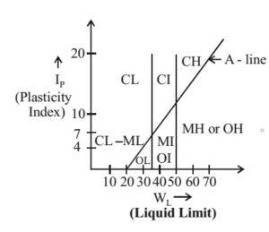
Plasticity Chart

Equation of A line is IP = 0.73 (W_L – 20) Note: I_P = 0, w_L = 20.

While drawing A line, it meets x-axis at 20.

When a question is asked with IP and WL to find the type of soil, draw the graph with A-line and locate the point on it with the given values of W_L and I_P see at which portion the point comes.

Representation

C – Inorganic Clay

M – Inorganic Silt

O – Organic clay/ Silt

L – Low compressible

I – Intermediate Compressible

H – High compressible

Example – CL means Low compressible inorganic clay. OH means High compressible organic clay/ silt.

PERMEABILITY

What is Permeability?

Permeability is the property of soil which permits the flow of water through its interconnected voids.

Darcy’s law :

Discharge, q = k.i.A

where k is Coefficient of permeability (cm/s or m/s or m/day)

i is hydraulic gradient or head loss/seepage length, i = Δh/l

A is Perpendicular cross sectional area

Discharge Velocity, V = q/A = k.i

Types of Soils and their values of K

Gravel – 1

Sand – 10^-2

Silt – 10^-4

Clay – 10^-6

Seepage Velocity, V_S = V/η

where η is porosity. Porosity will be always lesser than 1, so V_S is always greater than V

Factors Affecting Coefficient of Permeability

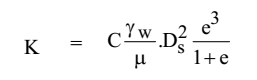
(Comparing Darcy’s and Poiseuille’s Equation)

k α γ_w where γ_wis unit weight of pore fluid
k α 1/µ → k₁/k₂ = µ₂/ µ₁ where µ is viscocity of pore fluid
k α e³/(1+e) ≈ e²→ k₁/k₂ = e₁²/e₂² where e is void ratio
k α D_S² where D_Sis diameter of grain.
According to Allen Hazen equation, K = CD₁₀² and C = 100 → K = 100D₁₀² where D₁₀ is effective diameter
k depends on shape of article
k is inversely proportional to specific surface area
k depends on method of compaction during deposition and structural arrangement of soil mass
Presence of undissolved gases, organic matter and other foreign matte

Determination of Coefficient of Permeability

– Laboratory methods

Constant Head Permeability Method – This method is suitable for sand.

k = qL/HA (q = k.i.A = k x h/L x A)

Where q is discharge, L is seepage length, H is Head Loss, A is perpendicular cross sectional area

Variable Head Permeability Test –This method is suitable for sand and silt.

k = aL/A x log_e(h₁/h₂)/(t₂-t₁) = 2.303 (aL/At) log₁₀(h₁/h₂)

where h₁and h₂ are head drops corresponding to time t₁ and t₂

a is area of stand pipe

A is cross sectional area of solid specimen

– Field Methods

Pumping out test
Pumping in test

– From the particle size

Using Allen Hazen equation, k = C.D_W² where C ≈ 100

– From consolidation test data (Suitable for clays)

– Capillarity (Permeability Test)

Aquifers

Confined Aquifer :

Discharge, q = 2.72(h₂-h₁)/log_e(r₂/r₁)

Where h₁and h₂ are depths of water in observation wells at distance of r₁and r₂ (r₂ > r₁ )

Unconfined Aquifer :

Discharge, q = 2.72k(H²-h²)/2log(R/r) = 1.36k(H²-h²)/log(R/r)

In Reccuperation test, specific yield k/A = 2.303 log(H₁/H₂)/T

Permeability of Stratified Deposit

Flow parallel to stratification plan

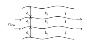
In this case, head loss and hydraulic gradient is constant.

Total Discharge Q = q₁ + q₂ + q₃ + ……..

Permeability K_H = k₁d₁+k₂d₂+…. / d₁+d₂+….

Flow perpendicular to stratification plane

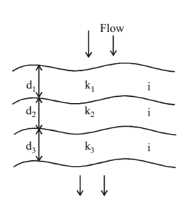
In this case, discharge is constant.

Total Head Loss, H = h₁+h₂+h₃+……

Permeability k_v = d₁+d₂+…./(∂₁/k₁+∂₂/k₂+…..)

i.e. d₁+d₂+d₃+…./k_v = d₁/k₁+ d₂/k₂ + ….

Note: Always k_H is greater than k_v. Flow parallel to stratification plane is governed by most permeable layer and flow perpendicular to stratification plane is governed by least permeable layer.

SEEPAGE

Percolation of water through soil pores due to an external force or energy gradient is known as seepage. Total head in soil causing seepage is the sum of pressure head and datum head (velocity head is neglected due to low velocity of percolation).

i.e., H = hw ± z

Hydraulic gradient (i)

It is the loss of head per unit seepage distance. i = h/L

Flowline (stream line)

Path along which water particle percolates is called flowline or streamline.

Equipotential line

Equipotential line is the line joining points of equal total head. In an equipotential line, total head is constant but pressure heads are different and datum heads are also different. A piezometer will rise to an equal elevation at all points in an equipotential line. This elevation is called piezometric level.

Flow net – Combination of flow lines and equipotential lines.

Flow path (flow channel) – Space between two adjacent flow lines.

Field – Space between two adjacent flow lines and adjacent equipotential lines. Flow lines are approximately squares in shape

Seepage quantity (discharge) – Total discharge through a flow net.

q = k.H.N_f/N_d

where k is coefficient of permeability, H is Head causing flow, N_f is Number of flow channels, N_d is Number of potential drops

Seepage Pressure (P_S) – It is the change in effective pressure due to seepage.

P_S = H.r_w = i.z.r_w

H is hydraulic potential after n potential drops

H = h – n.ΔH

ΔH = h/N_d

h — total head causing flow.

Seepage force per unit volume = i.r_w

Uplift Pressure (P_u)

At any depth, P_u = r_w.h_w

Where h_w is pressure head at that depth = total head – datum head

Exit gradient – It is the hydraulic gradient where percolating water leaves the soil mass and emerges into free water.

Exit gradient, i_e = ΔH/Δl

ΔH = h/N_d (potential/head drop)

Δl is the average length of last field at downstream end

Points to be noted

Flow lines and equipotential lines are perpendicular to each other.
Two flow lines or two equipotential lines never meet each other.
Drop in total head between adjacent equipotential lines is the same.
Flow net does not depend on permeability of soil (k) and head causing flow (H). It depends only on boundary conditions.
Quantity of seepage in each flow channel in the same.

QUICK SAND

What is Quick Sand?

Quick sand is a condition in fine sand that occurs when seepage is in the upward direction. When the seepage pressure acts in the upward direction and if it becomes equal to the submerged weight of soil, effective pressure becomes zero.

In this case, the cohesionless soil losses all its shear strength and it moves in upward direction.

This phenomenon is called quick sand condition/boiling condition.

Downward force = submerged weight of soil = γ’.H (H is thickness of soil)

Upward Force = seepage pressure = γ_w.h (h is head causing flow)

At quick sand condition, γ’.H = γ_w.h

Head Required for Quick Sand:

γ’.H = γ_w.h

Head required, h = γ’.H/ γ_w

If there is a surcharge, it is also a downward force against seepage.

Therefore, Total Downward Force = γ’.H + q

Head causing flow, h = (γ’.H + q)/γ_w

Critical Hydraulic Gradient (i_c) – Hydraulic gradient at quick sand condition is called critical hydraulic gradient. At quick sand condition, exit gradient is equal or just greater than critical hydraulic gradient.

i_c= h/H = γ’/γ_w = (G-1)/(1+e) = (G-1)(1-η)

h is head causing flow

H is thickness of sand

γ’= γ_sub

1/(1+e) = 1-η (Since e = η/1-η)

Special Case: When G=2.67 and e=0.67, i_c = (G-1)/(1+e) = (2.67-1)/(1+0.67) = 1

Points to be noted

Quick sand is not a type of sand. It is a phenomenon that occurs on sand and other cohensionless soil.
Quick sand condition occurs only in cohensionless soil (silt & fine sands)

PIPING

What is Piping phenomenon?

During quick sand condition, soil loses its shear strength and has the tendency to move in the direction of seepage flow. Thus the sand particles flows along with seepage water. This phenomenon is called piping. Piping is common in dams.

Factor of safety against quick sand/piping:

F = Critical hydraulic gradient/exit gradient = i_c/i_e

Seepage in anisotropic soil – When water seeps through soils of different permeabilities, the principle of square flow net is not valid.

Equivalent Permeability, k’ = Square root of k_x.k_y

When water flows from soil of one permeability to another, flow lines and equipotential lines gets deflected at the junction. Ratio of tangents of the angles made by these lines is equal to the ratio of permeabilities of the soils.

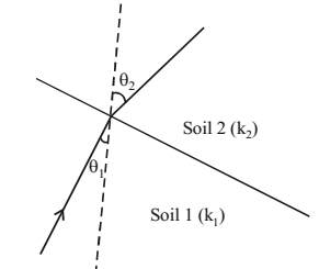
tanθ₁/tanθ₂ = k₁/k₂

EFFECTIVE STRESS

Total stress at base of soil column = Total force or load per unit area

σ = γ_sat x h

Pore water pressure/neutral stress (µ) – It is the pressure due to pore water in the voids.

µ = γ_w.h

Effective stress – It is the pressure exerted among the soil particles. So it is also called ‘intergranular pressure’

Points to be noted

Effective stress cannot be measured directly with a given soil. It can only be calculated from other quantities.
Effective stress in soil with varying water table levels. While calculating effective stress, we take bulk unit weight for soil above water table and saturated unit weight for soil below water table level.

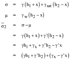
Consider an example. Let’s take datum xx at a distance (h₁ + h₂) from ground surface and water table level at depth of h₁ from surface.

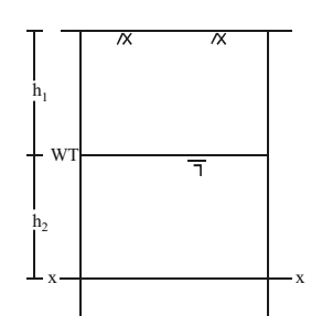
Total Stress, σ = γh₁+γ_sath₂

Pore Pressure, µ = γ_w.h₂

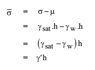
Effective Stress,

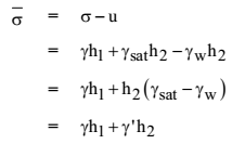
Now consider another case that water level was at a distance x from the previous case.

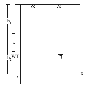
γ’ is always less than γ, hence (γ_x – γ’x) is a positive value

i.e., effective stress in 2nd case is more than that of first case. Therefore as water table gets depressed (comes down), effective stress increases and vice versa.

How to find effective stress in any case of datum and water table level

Consider individual heights of different layers of soil and multiply it by corresponding density values. For soil layers above water table take bulk unit weight (γ) and for soil layers below w.t. take saturated unit wt. (γ_sat).

To find pore water pressure, take sum of heights of soil layers from water table till datum and multiply by γ_w. If the section we consider is above water table level, pore water pressure is zero.

To find effective stress, take the difference of total stress and pore water pressure and remember γ_sat – γ_w = γ’ or γ_sub

Go through the below example.

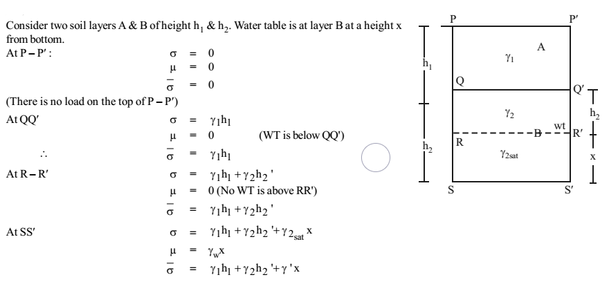
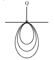
STRESS DISTRIBUTION

Consider a load Q acting on a soil layer. The vertical stress (V2) at a point P which is at a vertical distance z below the load and a radial distance of r, is given by Bousinesq’s equation

Points to be noted

Bousinesq’s equation is used mainly for shallow foundation
It is applicable to any soil at V2 does not depend on young’s modulus (E) and poisson’s ratio of soil.
Theoretically, V2 = 0 only at infinite distance but it becomes negligible after some distance below the surface.

Special Case – When the point P is on the vertical line of load Q, r=0

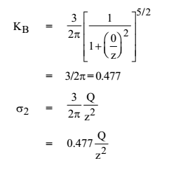
Variation of Vertical Stress

Case 1: Variation of σ₂ in horizontal direction

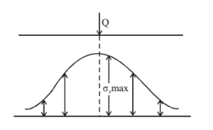
Case 2: Variation of V2 in vertical direction below the load

It varies parabolically as σ₂ α 1/z²

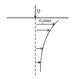
Case 3: Variation of V2 in vertical direction at a radial distance r from load

σ₂ is maximum when r/z = 0.817

β = tan^-1(r/z) = 39⁰15’

Isobar

What is an Isobar?

It is the contour connecting points of equal vertical stresses. The presence of soil inside an isobar is greater than pressure of soil outside that isobar. The zone in the soil mass surrounded by isobar is called pressure bulb.

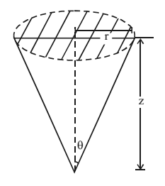
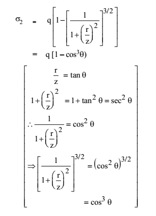
Vertical stress due to circular loaded area – Vertical stress at a point at depth z along the centre of circular area having radius ‘r’.

Newmarks influence chart

It is a chart based on Bousinesq’s theory which is used to find vertical stress below loaded area of dry shape.

Vertical stress, σ_z = I.n.q

Where I is Influenze coefficient (≈0.005 i.e., 5×10^-3)

n is number of sectors occupied by footing in the chart

q is Intensity of loading

Westergaards Theory – This is also used to find vertical stress which is suitable for stratified soil and clays.

σ_z= Q/z² x 1/π x [1/(1 + 2(r/z)²)]^3/2

Note : Note the three charges of this equation with the Bousinesq’s Equation.

CONSOLIDATION –

What is Consolidation?

Consolidation is the phenomenon of gradual compression of soil mass by expulsion of water from the voids/ pore due to long term static load/ pressure. This is different from compaction, as compaction is expulsion of air and is of shorter duration. Consolidation takes place in three stages of expulsion of air, water and high viscous liquids known as initial, primary and secondary consolidation respectively.

Terzaghi’s Piston and spring model

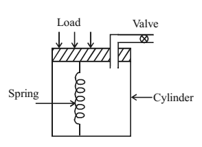
Actual Material/Property	Model
Soil Grains	Spring
Voids	Cylinder
Effective Stress in Soil	Load on Spring
Effective Pore pressure	Load on Water
Permeability	Valve

Compression Index (C_C) It is the slope of log of stress and void ratio graph.

C_C = (e₁ – e₁)/log₁₀(σ₁/σ₀)

Where e₀ and e₁ are initial and final void ratios (e₀ > e₁)

σ₀ and σ₁ are corresponding initial and final stresses (σ₁ > σ₀)

Determination of C_c

C_c = 0.007 (w_l – 10) For remoulded soil

C_c = 0.009 (w_c – 10) For undisturbed soil

w_l – liquid limit (in%)

Empirical formula C_c = 0.54 (e₀ – 0.35) where e₀ is in situ void ratio

Recompression Index (C_r)

Recompression is compression of soil which was already loaded and unloaded. This is much less compared to compression index.

Coefficient of Compressibility (a_v) – It is the, decrease in void ratio with unit increase in stress.

a_v = e₀-e₁/σ₁-σ₀

Coefficient of volume compressibility (m_v)

m_v = ΔV/V x 1/Δσ

For laterally confined soil, m_v = ΔH/H x 1/Δσ = Δe/1+e₀ x 1/Δσ

ΔH is called consolidation settlement (S_f)

Consolidation Settlement (S_f or DH)

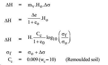
Δσ is increase in effective stress

Over Consolidation Ratio (OCR)

What is the Over Consolidation Ratio?

If a soil mass was subjected to higher pressure or stress (σ_c) in the past than the present pressure (σ), the ratio of that higher pressure to present pressure is called over consolidation ratio.

OCR = σ_c/σ

OCR will be less than 1, if there was no higher pressure acting on the soil than the present pressure acting on it (under consolidated soil).

Coefficient of consolidation (Cv)

Coefficient of consolidation, Cv is given by C_v = k/m_v.γ_w(m²/s)

Where k is coefficient of permeability

m_v is coefficient of compressibility

Time Factor (T_v)

Time factor (T_v) is given by, T_v= C_v.t/d²

Where C is coefficient of consolidation

t is Time taken for consolidation

d is drainage path

Value of d = H for single drainange, H/2 for double drainage

[This equation is important for gate exam and note the value of d. For double drainage it is not 2H but is H/2]. Time taken for consolidation, t is directly proportional to d²

t₁/t₂ = (d₁/d₂)²

C_vis constant for a soil and T_vis same for same degree of consolidation.

Determination of coefficient of consolidation

1. Square root time fitting method.

(T_v)₉₀ = C_vxt₉₀/d²

t₉₀ is time taken for 90% consolidation

2. Logarithmic time fitting method

C_v = (T_V)₅₀ x d² / t₅₀

(T_v)₅₀ is time factor for 50% consolidation = 0.197

Degree of Consolidation (u)

u = (Settlement at any time/Ultimate Settlement) x 100

= S/S_f x 100

U = Dissipated excess pore water pressure/Initial excess pore water pressure = (u_i-u/u_i) x 100

Where u_i is initial even pore water pressure and u is pore water pressure at given time

When u ≤ 60%, T_v = π/4 x (u/100)² (u in %)

When u > 60%, T_v= 1.781 – 0.933 log₁₀(100-u)

COMPACTION

What is Compaction?

Compaction is the process of increasing unit weight of soil by expulsion of air from the voids by applying an external force (rolling, tamping etc.)

Relation between dry density and water constant is γ_d = Gγ_w/1+e

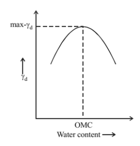
Optimum moisture content (OMC)

When water is added to dry soil, the adsorbed water acts as lubricant by forming a thin film around the soil grains. Thus on applying external load soil is well compacted and dry density gets increased. When the water content is increased, the water starts occupying the space between soil grains, hindering close packing of grains during compaction. Thus dry density decreases. Thus we have, to find the optimum water content at which we get maximum compaction and eventually the maximum dry density. This maximum dry density obtained is called proctor density. The amount of compactum and OMC is found by standard proctor compaction test or by modified proctor test (more efficient)

Zero air void line – It is the plot between dry unit weight and water content corresponding to 100% degree of saturation or zero air voids. Equation of zero air void line

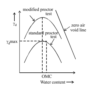
Equation of zero void line

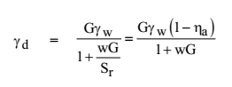
S_r = 100% , η_a = 0 and w is water content of compacted soil

Relative Compaction = (Dry Density in field/maximum dry density obtained) x 100

SHEAR STRENGTH

What is Shear Strength?

It is the resistance of shearing of soil particles when a shear stress acts on it, due to structural resistance due to interlocking, frictional resistance and cohesion.

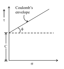
Mohr-coulomb theory – Shear strength (τ) is expressed as a function of normal stress (σ)

τ = C + σ.Tanφ

where c is apparent cohesion (kN/m²) and φ is angle of shearing resistance

Terzaghi’s theory – Shear stress (τ) is expressed as a function of effective normal stress (σ’)

τ = C’ + σ’ tanφ’

where C’ is effective cohesion, σ’ is effective stress (σ-u) and φ’ is angle of internal friction

Normal stress (σ’) and shear stress (τ) on any plane inclined at an angle α to the major principle plane can be expressed in terms of effective major principle stress σ’, and effective minor principle stress σ₃’

σ’ = (σ₁’+ σ₃’)/2 + (σ₁’- σ₃’)Cos2α/2

τ = (σ₁’- σ₃’)Sin2α/2

The graphical representation of these two equation give Mohr stress circle

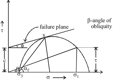
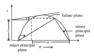
Critical shear plane – Critical shear plane is obtained from minimum difference (τ_f– τ) is taken we get.

α_f = 45 + φ/2

The critical shear plane is at an angle of α_f with major principle plane shown in figure.

Different types of tests for shear strength

Different types of tests are conducted for shear strength calculation based on the drainage condition.

Unconsolidated – undrained Test (UV – Test) or Quick test (Q–test) No drainage during both consolidation and shear stage. Takes only 5-10 minutes to complete. Example – unconfined compression test, Vane shear test
Consolidated – undrained test (Cu Test) or Rapid Test (R – Test) Drainage is permitted only in consolidation stage and not during shear stage.
Consolidated – Drained Test (CD test) or slow Test (S–Test) Drainage is permitted during both consolidation and shear stage. Taken 2–5 days to complete.

Points to be noted

For any combinations of σ₁’ and σ₃’ failure will occur only if mohr stress circle touches failure plane.

The shear stress at failure is less than maximum shear stress. i.e. failure plane does not carry maximum shear stress In terms of total stress,

τ_f = C_u + σ tan φ_u

where C_u is apparent cohesion and φ_u is apparent angle of shearing resistance.

DIFFERENT TEST FOR SHEAR STRENGTH

1. Direct shear Test – In direct shear test, for different values of vertical load, we find the failure shear stress and we plot the mohr circle with values of normal stress at each test. The shear strength parameters are then found out from the graph.

Shear strength, τ = c + σ tanφ

2. Triaxial Compression Test

Cell Pressure = σ₃ = σ_c = Confining pressure

Deviator stress, σ_d = σ₁ – σ₃

In the first staged this test, cell pressure (σ_c) is applied from all sides. In the second stage, deviator stress (σ_d) is given axially.

Thus, in axial direction total stress = σ_d + σ_c = σ₁– σ₃ + σ₃ = σ₁

Deviation stress, σ_d = additional axial load/area at failure or changed cross sectional area

= additional axial load/A’

A’ = V₁±ΔV/L₁-ΔL (drained triaxial test)

A’ = A₀/1-(ΔL/L)

Where A₀ is initial area, V₁ is initial volume, ΔV and ΔL are change in volume and length respectively

ΔL/L = e = axial strain

Tip: Remember the equations of cell pressure and deviator stress. Questions are usually asked from this equations.

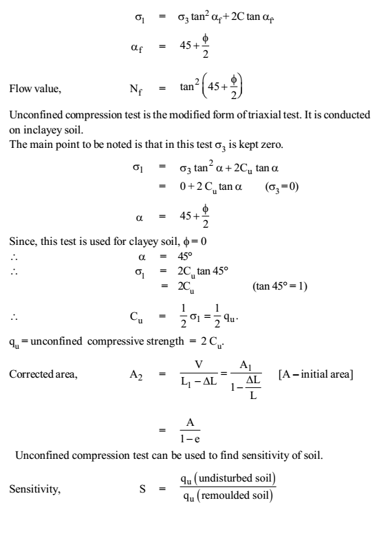
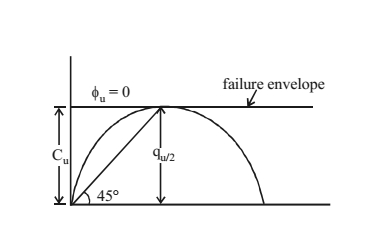
3. Unconfined compression test

Before going to the details of the test, it is important to know about plastic equilibrium.

Plastic Equilibrium – A material is said to be in plastic equilibrium when every point of it is at the verge of failure. The following equations are valid at plastic equilibrium.

4. Vane Shear Test

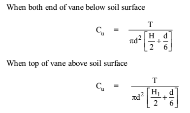
where,

T – torque

C_u – undrained cohesion of soil

H – height of vane

H₁ = height of vane below soil sample

d – diameter of vane

As per IS recommendation, H = 2d.

Tip: Check if the top end of vane is above or below soil when a question is asked about vane shear test. Remember to take H₁ in second case and not total height H.